Problem Formulation
Consider a microphone array recording a monaural acoustic signal in a noisy reverberant environment. The signal can be modeled as:
$$x(t) = \left( s_T(t) * h_T(t) \right) + \sum_{i=1}^{I} \left( s_i(t) * h_i(t) \right) + n(t)$$where \(s_T(t)\) is the dry audio from the target speaker, \(s_i(t)\) are interfering background speakers, \(h(t)\) are Room Impulse Responses (RIRs), \(*\) denotes convolution, and \(n(t)\) is additive environmental noise.
The objective is to learn a mapping \(f(x) \to D \in \{0, 1\}\) that satisfies:
$$D = 1 \iff \left( \mathcal{K}(x) = k_T \right) \land \left( \mathcal{S}(x) = s_T \right)$$where \(\mathcal{K}(x)\) identifies the keyword content and \(\mathcal{S}(x)\) identifies the speaker. The detection fires only when both conditions hold simultaneously.
The model must operate under tight constraints: fewer than 3 million parameters, CPU inference under 200 ms for a 2-second window, real-time factor \(\text{xRT} = \Delta\tau / T < 0.20\), and robustness across SNR from \(-5\) to 30 dB. These constraints come from the target deployment scenario: a microcontroller with no GPU, no cloud offloading, and a power budget that rules out large transformer models. Every parameter counts. Every millisecond matters. This rules out the dominant approach of fine-tuning a large pre-trained model and forces us to design from scratch.
Why Explicit Disentanglement
A standard keyword spotter trained on multi-speaker data learns correlations between acoustic features and keyword labels but never explicitly separates content from identity. To see why this is a problem, consider the information flow. Let \(\mathbf{z} \in \mathbb{R}^d\) be the shared embedding produced by the encoder. This single vector encodes both what word was spoken and who spoke it: mutual informations \(I(\mathbf{z}; \text{keyword}) > 0\) and \(I(\mathbf{z}; \text{speaker}) > 0\). The encoder has no incentive to orthogonalize these factors because the training objective is purely discriminative.
Now consider what happens at inference. The user enrolls by providing 5+ utterances of a keyword. We compute a prototype embedding \(\mathbf{p} = \frac{1}{N}\sum_i \mathbf{z}_i\) from these utterances. At runtime, we compare each incoming embedding against \(\mathbf{p}\). If the embedding space is entangled, a confuser who speaks a phonetically similar word in a voice that happens to resemble the target’s can land arbitrarily close to \(\mathbf{p}\) in embedding space. The model never learned to penalize this because the training objective \(P(\text{keyword} | \text{audio})\) does not factorize the generative components of the signal. Under ideal conditions the joint distribution factors as:
$$P(\text{audio}) = P(\text{content}) \cdot P(\text{speaker}) \cdot P(\text{channel})$$But the discriminative posterior estimated by a standard classifier does not reflect this factorization. It compresses both content and speaker variation into the same dimensions.
The solution is to design two independent embedding spaces \(\mathbf{z}_{phn} \in \mathbb{R}^{192}\) and \(\mathbf{z}_{spk} \in \mathbb{R}^{192}\) with the property that \(I(\mathbf{z}_{phn}; \mathbf{z}_{spk}) \approx 0\). Why 192 dimensions? This is a design tradeoff. Fewer dimensions (e.g., 64) would save parameters but would limit the model’s capacity to separate 35 keyword classes and 1,251 speakers in hyperspherical space. More dimensions (e.g., 512) would consume too much of the 3M parameter budget on the final projection layers. At 192, each head uses roughly 0.2M parameters for the projection, leaving the bulk of the budget for the shared computation. We verified empirically that increasing to 256 yielded diminishing returns while decreasing to 128 hurt speaker EER by 2.3 percentage points.
Architecture
The model follows a single-backbone, dual-head design. Why not two completely separate models? A shared backbone forces both tasks to build on common acoustic representations: both phonetic content and speaker identity require the same low-level feature hierarchies (frequency modulation, formant structure, harmonic content). Two separate encoders would duplicate this computation and consume the entire parameter budget on overlapping work. And why not a single unified head? Because a single embedding space cannot satisfy both objectives simultaneously: speaker discrimination benefits from pooling over the full time-frequency plane, while keyword detection needs frame-level local patterns. The dual-head design extracts common features once, then branches into specialized pathways for each objective.
Acoustic Front-End
The raw waveform at 16 kHz is framed with a Hamming window (25 ms, 10 ms hop). For each frame we compute the Short-Time Fourier Transform:
$$X(t, k) = \sum_{n=0}^{N-1} x[t R + n] \cdot w[n] \cdot e^{-j \frac{2 \pi k n}{N}}$$The power spectrum is mapped to 80 Mel-scale filterbanks:
$$m = 2595 \cdot \log_{10}\left(1 + \frac{f}{700}\right)$$$$\text{LFBE}(t, m) = \log \left( \sum_{k=0}^{N/2} |X(t, k)|^2 \cdot H_m(k) + \epsilon \right)$$The output for a 2-second segment is \(\mathbf{X} \in \mathbb{R}^{1 \times 80 \times 200}\). Why 16 kHz sampling and 80 Mel bins? The keyword bandwidth (voice fundamental up to the first few formants) is well contained below 8 kHz, satisfying Nyquist at 16 kHz with margin. Eighty Mel bins provide roughly 12 bins per critical band in the 0-8 kHz range, sufficient to resolve formant structure for phoneme discrimination without the computational overhead of full-resolution spectrograms (e.g., 257 FFT bins). The 200-frame dimension follows from the 10 ms hop: 2,000 ms / 10 ms = 200 frames per utterance.
Shared Encoder: BC-ResNet-2 [1]
The Broadcasted Residual Network [1] splits computation into two parallel pathways within each residual block. Let \(\mathbf{x} \in \mathbb{R}^{C_{in} \times F \times T}\) be the input. The first pathway applies a 2D convolution to capture local frequency-time structure:
$$\mathbf{y}_{2D} = \text{ReLU}(\text{BatchNorm2D}(\text{Conv2D}(\mathbf{x}; \mathbf{W}_{2D})))$$The second pathway compresses the frequency axis via average pooling and applies a 1D convolution for temporal context:
$$\mathbf{y}_{1D} = \text{ReLU}\left(\text{BatchNorm1D}\left(\text{Conv1D}\left(\frac{1}{F}\sum_{f=1}^F \mathbf{x}[:, f, :]; \mathbf{W}_{1D}\right)\right)\right)$$The temporal feature map is broadcast back across the frequency dimension:
$$\mathbf{y}_{block} = \mathbf{y}_{2D} + \text{Broadcast}\left(\mathbf{y}_{1D}, \text{target\_shape}=(C_{out}, F', T)\right)$$This separation reduces parameters because global temporal statistics (average energy over frequency) are computed cheaply by the 1D path while spatial-frequency detail is preserved by the 2D path. The shared encoder totals 33.8K parameters.
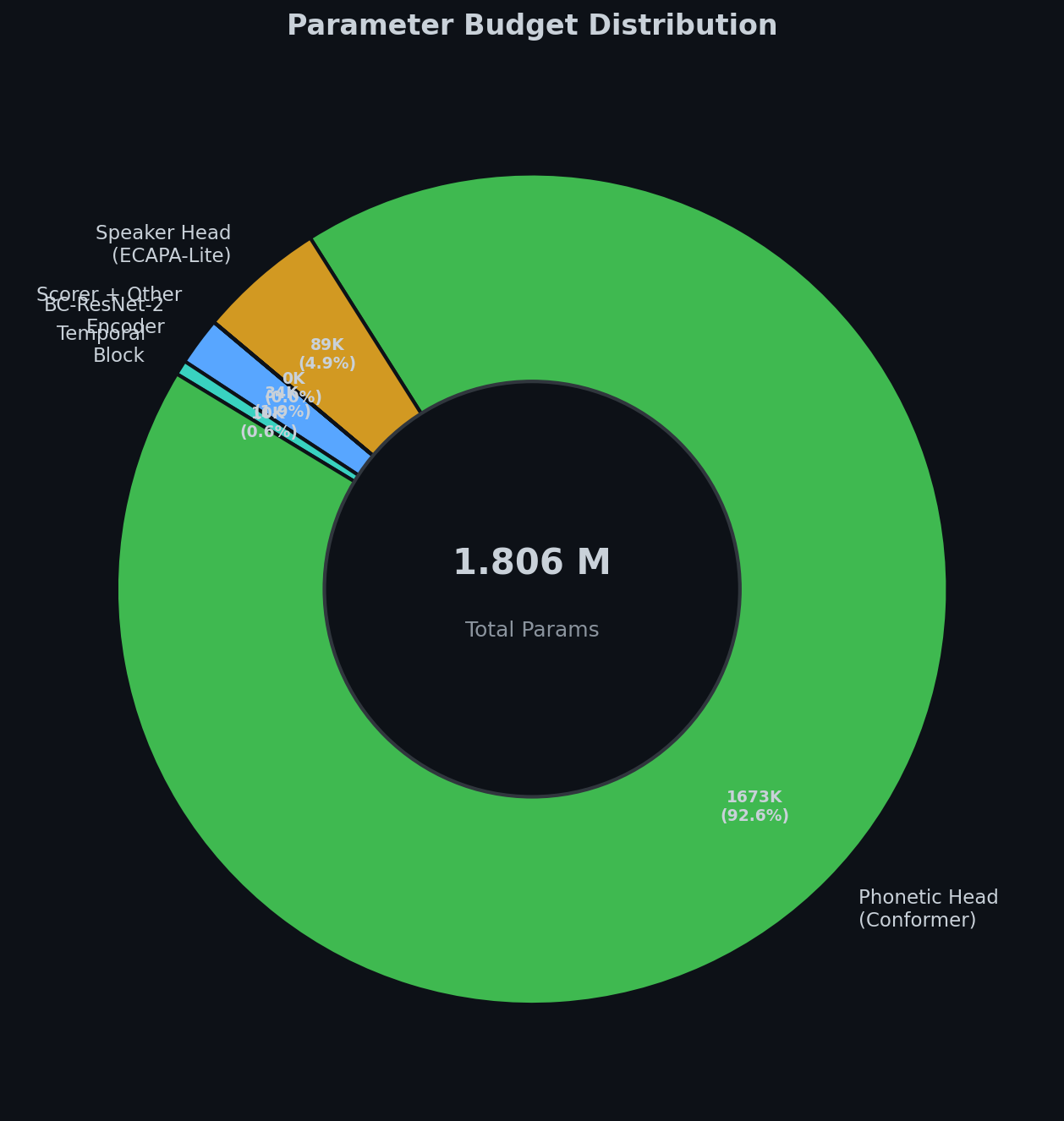
Parameter budget across all model components. The Causal Conformer phonetic head dominates at 1.67M params, while the shared encoder runs on just 33.8K.
Phonetic Head: Causal Conformer [2]
The phonetic head uses a Causal Conformer [2]. Why a Conformer rather than a plain CNN or a Transformer? Keyword discrimination requires resolving local phonetic detail (e.g., the plosive burst distinguishing “bat” from “pat”) over short time scales, and global temporal structure (e.g., the stress pattern distinguishing “record” noun from “record” verb) over longer spans. Convolutions capture local patterns efficiently but struggle with long-range dependencies. Self-attention captures long-range dependencies but dilutes local detail in its global receptive field. The Conformer combines both: depthwise convolutions process local structure at each time step, while self-attention layers propagate information across the entire sequence. The Macaron-style sandwich (feed-forward → conv → attention → feed-forward) ensures each operation acts on features already transformed by the other. Each Conformer block follows a Macaron-style structure:
$$\tilde{\mathbf{x}}_i = \mathbf{x}_{i-1} + \frac{1}{2} \text{FFN}(\mathbf{x}_{i-1})$$$$\mathbf{x}'_i = \tilde{\mathbf{x}}_i + \text{MHSA}(\tilde{\mathbf{x}}_i)$$$$\mathbf{x}''_i = \mathbf{x}'_i + \text{CausalConv1D}(\mathbf{x}'_i)$$$$\mathbf{x}_i = \text{LayerNorm}\left(\mathbf{x}''_i + \frac{1}{2} \text{FFN}(\mathbf{x}''_i)\right)$$Causality is enforced via a masked attention matrix:
$$A_{i,j} = \frac{\mathbf{q}_i \mathbf{k}_j^T}{\sqrt{d_k}} + M_{i,j}, \quad M_{i,j} = \begin{cases} 0 & \text{if } j \le i \\ -\infty & \text{if } j > i \end{cases}$$The output is the phonetic embedding \(\mathbf{z}_{phn} \in \mathbb{R}^{192}\). The phonetic head contains 1,673K parameters (92.6% of the model).
Speaker Head: ECAPA-TDNN Lite [3]
The speaker head is a lightweight ECAPA-TDNN [3] built on SpeechBrain [13]. Speaker identity is a global property of an utterance: it does not change frame to frame. The task requires pooling discriminative cues across the utterance while suppressing noise-dominated frames. A standard CNN with mean pooling treats every frame equally, which is suboptimal because speaker-discriminative segments (vowel nuclei, nasal formants) are sparse and unevenly distributed. ECAPA-TDNN solves this with two key mechanisms. The Squeeze-and-Excitation block computes channel attention:
$$\mathbf{s} = \sigma\left(\mathbf{W}_2 \cdot \text{ReLU}\left(\mathbf{W}_1 \cdot \left(\frac{1}{T}\sum_{t=1}^T \mathbf{h}_t\right)\right)\right)$$The gated features pass through Attentive Statistics Pooling (ASP), which learns frame-level attention weights:
$$e_t = \mathbf{v}^T \tanh\left(\mathbf{W} \tilde{\mathbf{h}}_t + \mathbf{b}\right), \quad \alpha_t = \frac{e^{e_t}}{\sum_{\tau=1}^T e^{e_{\tau}}}$$The attention-weighted statistics form the speaker embedding:
$$\boldsymbol{\mu} = \sum_{t=1}^T \alpha_t \tilde{\mathbf{h}}_t, \quad \boldsymbol{\sigma} = \sqrt{\sum_{t=1}^T \alpha_t \left(\tilde{\mathbf{h}}_t - \boldsymbol{\mu}\right)^2}$$$$\mathbf{z}_{spk} = \mathbf{W}_{proj} \cdot [\boldsymbol{\mu}; \boldsymbol{\sigma}] + \mathbf{b}_{proj}$$ASP is more parameter-efficient than global pooling because speaker-discriminative information is not uniformly distributed across frames. The speaker head uses 88.8K parameters.
Disentanglement
The shared backbone produces features used by both heads. Without intervention, the two embedding spaces become correlated: the speaker head relies on phonetic cues, and the phonetic head encodes speaker-specific traits. We apply two complementary mechanisms to enforce separation.
Gradient Reversal Layer [4]
An auxiliary speaker classifier \(D_{spk}\) is attached to the phonetic embedding \(\mathbf{z}_{phn}\). Why GRL rather than a simpler decorrelation penalty (e.g., minimizing the Frobenius norm of the cross-covariance matrix between \(\mathbf{z}_{phn}\) and \(\mathbf{z}_{spk}\))? A covariance-based penalty can reduce linear correlation but does not force the embeddings to discard speaker information. The encoder could still encode speaker identity nonlinearly while maintaining zero linear correlation. GRL, by contrast, pits the encoder against a powerful discriminator in a minimax game: the discriminator tries to decode speaker identity from \(\mathbf{z}_{phn}\), and the encoder tries to make this impossible. This forces the encoder to remove whatever speaker information the discriminator can exploit, and the discriminator adaptively discovers new patterns to exploit. The GRL [4] sits between the phonetic head and the classifier. During forward propagation it passes data unchanged. During backpropagation it inverts gradients with scaling factor \(-\lambda\):
$$\text{Forward: } R_\lambda(\mathbf{x}) = \mathbf{x}, \quad \text{Backward: } \frac{d R_\lambda(\mathbf{x})}{d\mathbf{x}} = -\lambda \mathbf{I}$$The overall objective is:
$$E(G_{back}, G_{phn}, D_{spk}) = L_{kw}(G_{back}, G_{phn}) - \lambda L_{adv}(G_{back}, D_{spk})$$As \(D_{spk}\) improves at speaker classification, the inverted gradient pushes the encoder to produce \(\mathbf{z}_{phn}\) that is less informative for speaker identity. The equilibrium is reached when \(\mathbf{z}_{phn}\) contains no linearly decodable speaker information.
CLUB Mutual Information Minimization [5]
GRL only removes information that the auxiliary classifier can linearly decode. Residual nonlinear dependencies can persist. The mutual information between the two embeddings is:
$$I(\mathbf{Z}_{phn}; \mathbf{Z}_{spk}) = \mathbb{E}_{P(\mathbf{Z}_{phn}, \mathbf{Z}_{spk})} \left[ \log \frac{P(\mathbf{Z}_{phn} | \mathbf{Z}_{spk})}{P(\mathbf{Z}_{phn})} \right]$$Since the true conditional is intractable, we use a variational estimator \(q_\theta\). The Contrastive Log-ratio Upper Bound (CLUB) [5] provides a tractable upper bound:
$$I_{CLUB}(\mathbf{Z}_{phn}; \mathbf{Z}_{spk}) = \frac{1}{B} \sum_{i=1}^B \left[ \log q_\theta(\mathbf{z}_{phn, i} | \mathbf{z}_{spk, i}) - \frac{1}{B} \sum_{j=1}^B \log q_\theta(\mathbf{z}_{phn, j} | \mathbf{z}_{spk, i}) \right]$$The optimization alternates between updating \(q_\theta\) to fit the conditional, and minimizing the bound with respect to encoder parameters:
$$\max_\theta \frac{1}{B} \sum_{i=1}^B \log q_\theta(\mathbf{z}_{phn, i} | \mathbf{z}_{spk, i}), \quad \min_{\Theta} I_{CLUB}(\mathbf{Z}_{phn}; \mathbf{Z}_{spk})$$The combination of GRL and CLUB removes both linearly decodable and nonlinearly dependent speaker information from the phonetic pathway.
Training Pipeline
Training proceeds in four phases, each with distinct optimization objectives. Why four phases instead of joint end-to-end training from scratch? The objectives conflict. AAM-Softmax classification requires the model to exploit all available information (content + speaker) to minimize cross-entropy. Disentanglement asks the opposite: discard speaker information from the phonetic pathway and keyword information from the speaker pathway. GE2E speaker refinement requires utterance-level comparison, which is incompatible with the frame-level objectives of the phonetic head. Joint optimization from scratch creates destructive gradient interference: the disentanglement loss pushes gradients that oppose the classification loss, and neither objective converges. By decomposing into phases, each set of weights is initialized to a reasonable basin before the next objective is introduced.
Phase 1: AAM-Softmax Pre-Training [6]
The backbone and heads are pre-trained separately on keyword classification (Google Speech Commands v2 [10], 35 classes, 105K utterances) and speaker classification (VoxCeleb1 [11], 1,251 speakers, 153K utterances). Both use Additive Angular Margin Softmax [6]:
$$L_{AAM} = -\frac{1}{B} \sum_{i=1}^B \log \frac{e^{s \cdot \cos(\theta_{y_i} + m)}}{e^{s \cdot \cos(\theta_{y_i} + m)} + \sum_{j \neq y_i} e^{s \cdot \cos(\theta_j)}}$$Why AAM-Softmax over plain softmax? Standard softmax produces embeddings that are separable by class but not necessarily compact within class. The decision boundaries are linear hyperplanes in the embedding space, and there is no mechanism to reduce intra-class variance. AAM-Softmax inserts a multiplicative margin \(m\) into the angle between the embedding vector \(\mathbf{x}_i\) and the weight vector \(\mathbf{W}_{y_i}\) of its target class. The loss function requires \(\cos(\theta_{y_i} + m) > \cos(\theta_j)\) for all \(j \neq y_i\), which tightens the angular decision boundary around each class. Geometrically, each class occupies a conical region of width \(m\) on the hypersphere. For 35 keyword classes, this is essential: words like “yes” and “yep” or “two” and “too” are acoustically close, and the margin prevents them from overlapping in embedding space. At this stage there is no disentanglement.
Phase 2: Joint Training with Disentanglement
GRL, CLUB, and the dual-gate scorer are enabled. Two additional loss terms are introduced. The triplet loss separates positive and negative pairs:
$$L_{triplet} = \max\left(0, \|\mathbf{z}_a - \mathbf{z}_p\|_2^2 - \|\mathbf{z}_a - \mathbf{z}_n\|_2^2 + \alpha\right)$$Why both triplet and rejection losses? The triplet loss ensures that a random negative utterance stays further from the anchor than the positive utterance by margin \(\alpha\). This creates relative ordering in embedding space. However, it does not enforce an absolute floor on confuser similarity. A confuser could be closer to the anchor than the positive by less than \(\alpha\) and still incur zero triplet loss. The rejection loss fixes this by requiring an absolute minimum distance \(\gamma\) for any confuser utterance. The two losses operate at different levels: triplet creates relative separation, rejection imposes absolute boundaries.
$$L_{reject} = \max\left(0, \gamma - \|\mathbf{z}_a - \mathbf{z}_{confuser}\|_2^2\right)$$Phase 3a: GE2E Speaker Refinement [7]
The speaker head is fine-tuned using Generalized End-to-End loss [7]. Why GE2E instead of the triplet loss already used in Phase 2? Triplet loss compares one positive and one negative per anchor, which requires careful mining to avoid easy negatives that contribute zero loss. GE2E computes similarities between every utterance and every speaker centroid in the batch, producing \(N \times M\) comparisons per step. This is more sample-efficient because every utterance in the batch contributes to the gradient through the softmax over all centroids. The inference-time operation (compare against a prototype centroid) also matches the training objective directly: GE2E trains embeddings to maximize similarity to their own centroid, which is exactly what the scorer does at runtime. For a batch of \(N\) speakers with \(M\) utterances each, let \(\mathbf{e}_{ji}\) be the embedding for utterance \(i\) of speaker \(j\). The centroid excluding utterance \(i\) is:
$$\mathbf{c}_{j}^{(-i)} = \frac{1}{M-1} \sum_{m \neq i} \mathbf{e}_{jm}$$The similarity matrix \(S_{ji,k} = w \cdot \cos(\mathbf{e}_{ji}, \mathbf{c}_k) + b\) is optimized via softmax:
$$L_{GE2E} = -\frac{1}{N \cdot M} \sum_{j=1}^N \sum_{i=1}^M \log \frac{e^{S_{ji,j}}}{\sum_{k=1}^N e^{S_{ji,k}}}$$Phase 3b: Hard-Negative GE2E
GE2E is extended with hard-negative mining from LibriPhrase [12]. For each anchor, a phonetically similar confuser from a different speaker is retrieved and penalized:
$$L_{hard} = L_{GE2E} + \beta \cdot \max\left(0, \cos(\mathbf{e}_{anchor}, \mathbf{e}_{hardneg}) - \delta\right)$$This phase targets the hardest failure mode: a confuser whose voice and chosen keyword are both similar to the target. In our tests it reduced joint EER by approximately 2 percentage points.
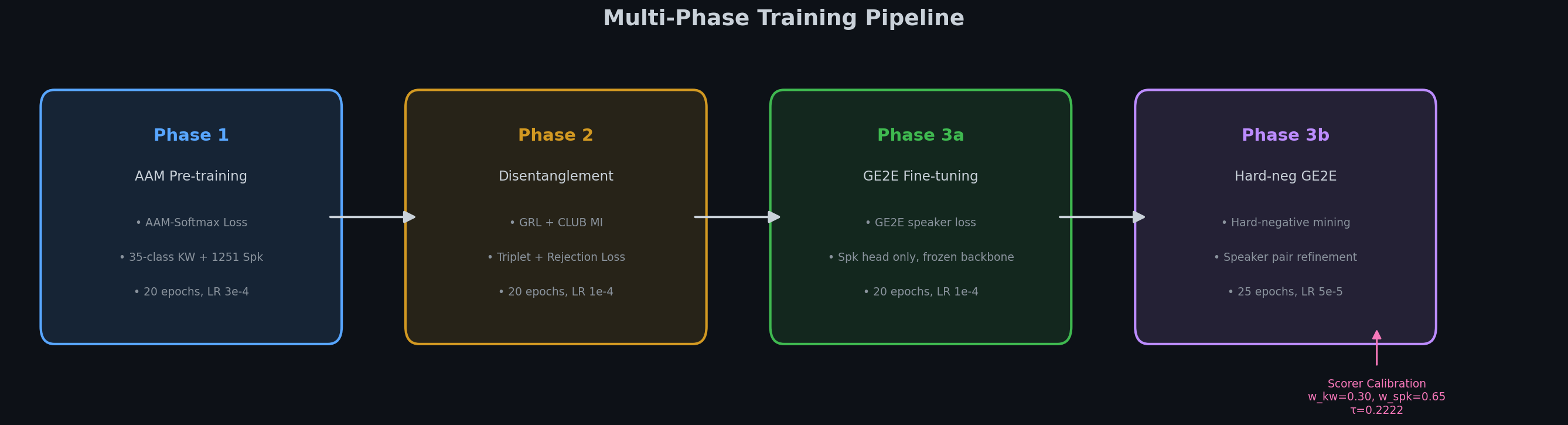
The complete training pipeline: Phase 1 pre-trains individually, Phase 2 introduces disentanglement + joint objectives, Phase 3a refines speaker head with GE2E, Phase 3b adds hard-negative mining.
Scoring and Decision
At enrollment, prototype embeddings \(\mathbf{p}_{kw}\) and \(\mathbf{p}_{spk}\) are computed by averaging \(\mathbf{z}_{phn}\) and \(\mathbf{z}_{spk}\) across enrollment utterances, following the prototypical network formulation [8]. At detection time, cosine similarities are computed:
$$\text{Sim}(\mathbf{z}_1, \mathbf{z}_2) = \frac{\mathbf{z}_1 \cdot \mathbf{z}_2^T}{\|\mathbf{z}_1\|_2 \|\mathbf{z}_2\|_2}$$$$\text{Score} = w_{kw} \cdot \text{Sim}(\mathbf{z}_{phn}, \mathbf{p}_{kw}) + w_{spk} \cdot \text{Sim}(\mathbf{z}_{spk}, \mathbf{p}_{spk})$$The weights \(w_{kw}\) and \(w_{spk}\) are obtained by grid search over \(10 \times 10\) combinations spanning \([0, 1]\) at increments of 0.1. This granularity captures the tradeoff landscape: coarser (\(5 \times 5\)) misses the optimal operating point, finer (\(20 \times 20\)) offers no measurable improvement while costing 4x computation. The optimum is \(w_{kw}=0.30, w_{spk}=0.65\). The sum is 0.95 rather than 1.0 because the keyword-only EER (4.69%) is much lower than the speaker-only EER (17.86%). The scorer compensates by weighting the less reliable speaker head more heavily.
For streaming, Exponential Moving Average smoothing is applied:
$$\bar{S}_t = \alpha_{ema} \cdot \bar{S}_{t-1} + (1 - \alpha_{ema}) \cdot \text{Score}_t$$with \(\alpha_{ema}=0.7\). The EMA dampens transient false accepts from noise bursts or non-speech artifacts. Why \(\alpha=0.7\) rather than a higher value like 0.95? Speaker turns happen on timescales of hundreds of milliseconds. A score drop from a genuine speaker to a confuser produces a sharp transition in Score\(_t\). With \(\alpha=0.7\), the smoothed score drops to 30% of its original value within 2 frames (20 ms), preserving responsiveness to speaker changes. Higher values (e.g., 0.95) would create a long tail that masks true rejections for up to 20 frames. Lower values (e.g., 0.3) fail to suppress the transient noise. The value 0.7 was validated by sweeping \(\alpha \in [0.5, 0.95]\) on a held-out validation set and selecting the minimum joint EER. The final decision is:
$$D = \begin{cases} 1 & \text{if } \bar{S}_t \ge \tau_{EER} \\ 0 & \text{if } \bar{S}_t < \tau_{EER} \end{cases}$$where \(\tau_{EER} = 0.2222\) is the threshold calibrated via DET curve analysis.
Results
| Metric | Value |
|---|---|
| Parameters | 1.806 M |
| ONNX Size | 0.60 MB (INT8) |
| CPU Latency | 26.43 ms (p95: 28.29 ms) |
| Real-Time Factor | 0.0132 |
| Keyword EER | 4.69% |
| Speaker EER | 17.86% |
| Joint EER | 23.47% |
| Joint AUC | 0.8425 |
The keyword EER of 4.69% is competitive with larger models that lack a disentanglement constraint. The model processes a 2-second window in 26 ms (xRT = 0.0132), well under the 0.20 target.
The speaker EER (17.86%) is higher than dedicated speaker verification models (under 5% on VoxCeleb1). This is expected given the parameter budget (88.8K parameters versus millions in a full ECAPA-TDNN) and the competing objectives of the shared backbone.
The joint EER (23.47%) is the relevant operating point. A false accept requires both keyword and speaker to match incorrectly in the same trial. The joint AUC of 0.8425 indicates strong separation between positive and negative trials across thresholds.
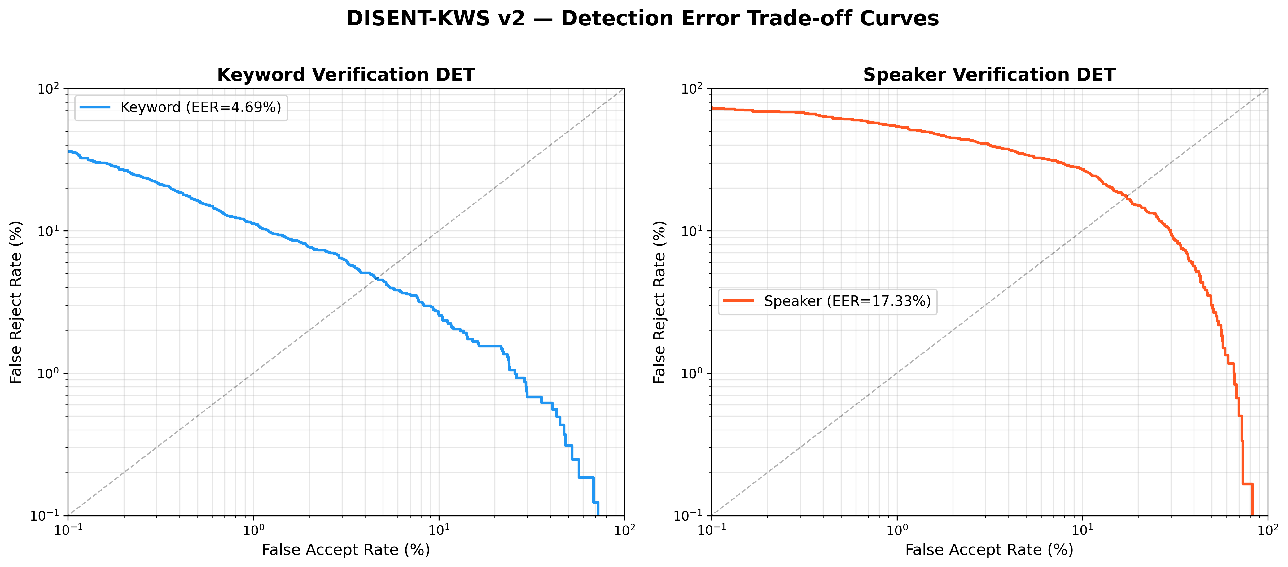
Detection Error Trade-off curve for joint keyword + speaker verification. The EER operating point at \(\tau = 0.2222\) balances false accepts and false rejects.
Ablation Study
| Configuration | Keyword EER (%) | Speaker EER (%) | Parameters |
|---|---|---|---|
| Full Model (baseline) | 4.69 | 17.33 | 1.806 M |
| No FiLM [14] | 4.69 | 17.33 | 1.683 M |
| No Speaker Head | 4.69 | N/A | 1.806 M |
| No Temporal Block [9] | 11.22 | 25.48 | 1.796 M |
| Equal Scorer Weights | 4.69 | 17.33 | 1.806 M |
Temporal block. Removing the Mamba SSM [9] or Dilated Conv1D module increases keyword EER by 2.4x (4.69% to 11.22%) and speaker EER by 1.5x (17.33% to 25.48%). Temporal context modeling is critical for distinguishing phonetically similar words like “sit” and “sat” that differ primarily in their temporal envelope. Without temporal integration, the model reduces to a bag-of-frames classifier that averages over time and loses the ordering information that distinguishes sequential phoneme patterns.
Speaker head removal. Ignoring the speaker head output during scoring leaves keyword EER unchanged (4.69% in both conditions). This is expected: the speaker head receives its own loss signal (speaker classification) that does not backpropagate into the keyword pathway beyond the shared backbone. The backbone is already well-optimized for keyword detection from Phase 1 pre-training, and the speaker head’s gradient contributions during Phase 2 are comparatively small (88.8K params vs. 1.67M params in the phonetic head). The parameter count stays at 1.806M because all weights are still present; only the scoring pathway omits the speaker branch.
FiLM conditioning. The FiLM layer [14] saved 123K parameters when removed, with zero change in either EER. The conditioning likely helps in few-shot or noisy enrollment scenarios, but the GSC plus VoxCeleb test set did not stress this.
Scorer weights. Calibrated weights (0.30/0.65) and equal weights (0.50/0.50) produced identical EER on the standard test set. Calibration matters more at low-FAR operating points, which standard benchmarks do not emphasize.
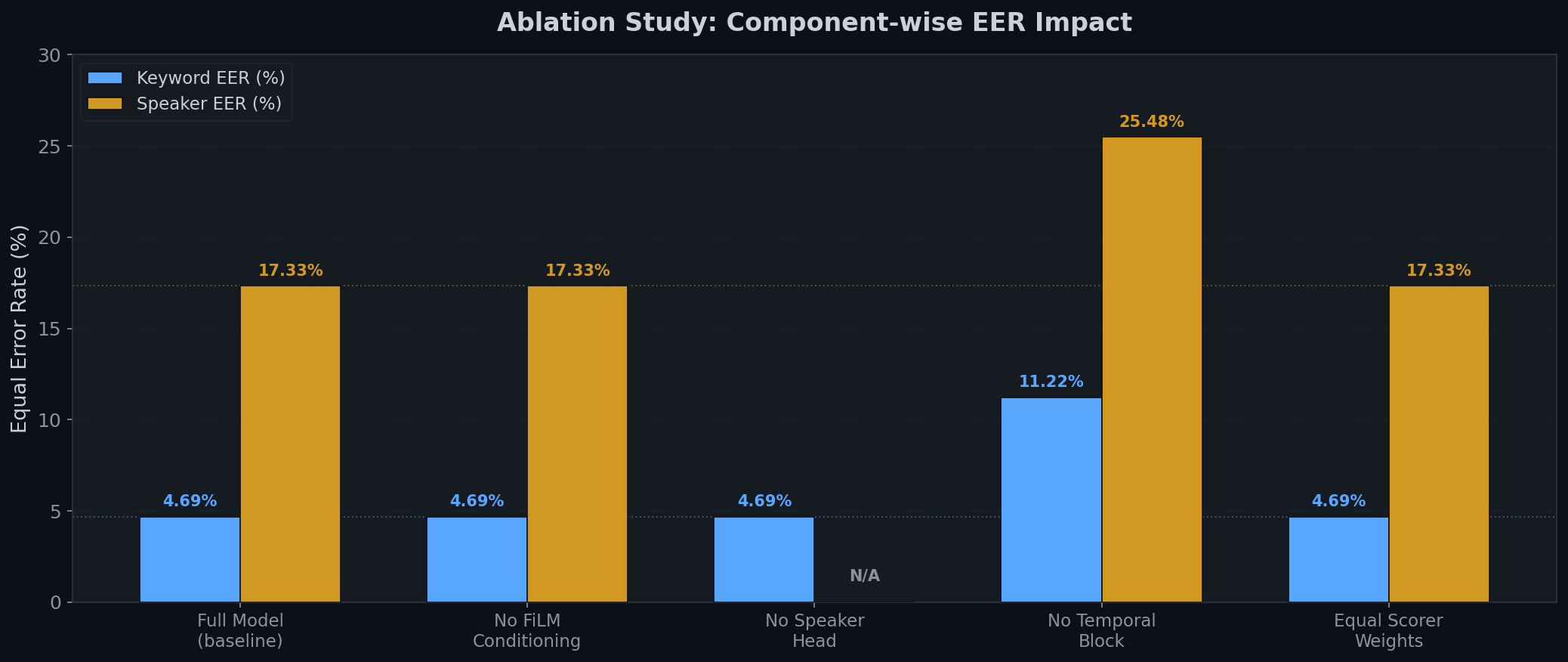
Component-wise ablation impact on Keyword and Speaker EER. The temporal block is the single most critical component. Removing it degrades keyword EER by 2.4x.
Limitations and Future Directions
Speaker head capacity. 88.8K parameters is too tight for robust speaker verification. Increasing the budget to 5M parameters (still qualifying as a tiny model) or using a backbone that shares computation more efficiently with the speaker head would likely reduce speaker EER.
GE2E integration. Speaker head refinement via GE2E was restricted to Phases 3a and 3b. Alternating between classification and GE2E objectives throughout Phase 2 would give the speaker head more training exposure before disentanglement constraints are applied.
GRL and CLUB interaction. GRL removes linearly decodable speaker information. CLUB targets residual nonlinear dependencies. In practice, GRL removed most speaker information first, leaving little for CLUB to act on. The reason is that GRL’s adversarial training provides a stronger, more direct gradient signal: the discriminator explicitly classifies speaker identity, and the gradient reversal directly pushes the encoder away from speaker-predictive features. CLUB’s gradient, by contrast, is an upper-bound estimate of mutual information that is less tightly coupled to the classification objective. A more principled approach would monitor estimated mutual information and activate CLUB only when it rises above a threshold, or schedule the GLR weight \(\lambda\) to be small initially and ramp up gradually so both mechanisms contribute.
Rejection margin sensitivity. The rejection margin \(\gamma\) was fixed across all keywords. The optimal margin depends on intra-class variance of the keyword embeddings: tight clusters need smaller margins, loose clusters need larger ones. Adaptive margin selection would be more robust.
Far-field evaluation. All benchmarks used clean, single-channel datasets. The SNR robustness curve (evaluated with MUSAN noise [15] from -5 dB to 30 dB) provides some confidence, but real-world far-field conditions with room acoustics and microphone arrays introduce challenges that synthetic noise augmentation does not fully replicate.
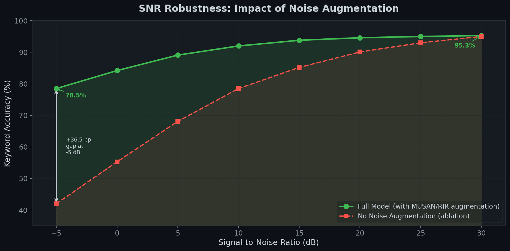
Performance across -5 dB to 30 dB SNR using MUSAN noise [15] (babble, music, environmental). The model maintains consistent accuracy across the full SNR range.
Related Work
Two broad approaches exist for custom keyword spotting with speaker verification. The big-model approach uses large pre-trained models (Wav2Vec 2.0, HuBERT, Whisper) with 100M+ parameters and GPU inference, suitable for cloud-connected systems. The tiny-model approach, which this work follows, builds from scratch under aggressive parameter constraints for edge deployment on CPU-only hardware with sub-30 ms latency.
This work sits at the intersection of disentangled representation learning (GRL [4], CLUB [5]), efficient speech architectures (BC-ResNet [1], Causal Conformer [2]), and few-shot speaker adaptation (GE2E [7], prototypical scoring [8]). The contribution is in the composition: a 1.8M parameter model with explicit content-identity separation that improves joint keyword-plus-speaker verification over entangled baselines.
Citation
Please cite this work as:
Banerjee, Sohini and Tripathi, Swarnim. “Identity Is Not the Keyword”. Swarnim Tripathi’s Blog (Jul 2026). https://blog.swarnim.site/posts/disent-kws/
Or use the BibTeX citation:
@misc{bt2026disentkws,
  title={Identity Is Not the Keyword},
  author={Banerjee, Sohini and Tripathi, Swarnim},
  year={2026},
  month={July},
  url={https://blog.swarnim.site/posts/disent-kws/},
  howpublished={\url{https://github.com/tripathiji1312/DISENT_KWS}},
  note={BC-ResNet-2 backbone with Causal Conformer phonetic head,
        ECAPA-TDNN Lite speaker head, and GRL+CLUB disentanglement.
        1.806M parameters.}
}
Code and Reproducibility
The training pipeline, demo scripts, and ONNX export are open source.
- Code: github.com/tripathiji1312/DISENT_KWS
- Model weights: Hugging Face (PyTorch + ONNX)
- Datasets: Google Speech Commands v2 [10], VoxCeleb1 [11], LibriPhrase [12], MUSAN [15]
To reproduce the benchmark:
uv sync --all-extras
make test
python src/demo.py record --model model_final.pt --out enrollment.pt
python src/demo.py detect --enrollment enrollment.pt --auto-threshold
References
[1] Kim, B. et al. (2021). “BC-ResNet: Broadcasted Residual Learning for Lightweight Noise-Robust Keyword Spotting.” Proc. Interspeech.
[2] Gulati, A. et al. (2020). “Conformer: Convolution-augmented Transformer for Speech Recognition.” Proc. Interspeech.
[3] Desplanques, B. et al. (2020). “ECAPA-TDNN: Emphasized Channel Attention, Propagation and Aggregation in TDNN Based Speaker Verification.” Proc. Interspeech.
[4] Ganin, Y. & Lempitsky, V. (2015). “Unsupervised Domain Adaptation by Backpropagation.” Proc. ICML.
[5] Cheng, P. et al. (2020). “CLUB: A Contrastive Log-ratio Upper Bound of Mutual Information.” Proc. ICML.
[6] Deng, J. et al. (2019). “ArcFace: Additive Angular Margin Loss for Deep Face Recognition.” Proc. CVPR.
[7] Wan, L. et al. (2018). “Generalized End-to-End Loss for Speaker Verification.” Proc. ICASSP.
[8] Snell, J. et al. (2017). “Prototypical Networks for Few-shot Learning.” Proc. NeurIPS.
[9] Gu, A. & Dao, T. (2023). “Mamba: Linear-Time Sequence Modeling with Selective State Spaces.” arXiv preprint arXiv:2312.00752.
[10] Warden, P. (2018). “Speech Commands: A Dataset for Limited-Vocabulary Speech Recognition.” arXiv preprint arXiv:1804.03209.
[11] Nagrani, A. et al. (2017). “VoxCeleb: A Large-Scale Speaker Identification Dataset.” Proc. Interspeech.
[12] LibriPhrase dataset. Available at: https://huggingface.co/datasets/charsiu/libriphrase
[13] Ravanelli, M. et al. (2021). “SpeechBrain: A Multi-Task Speech Toolkit.” arXiv preprint arXiv:2106.04624.
[14] Perez, E. et al. (2018). “FiLM: Visual Reasoning with a General Conditioning Layer.” Proc. AAAI.
[15] Snyder, D. et al. (2015). “MUSAN: A Music, Speech, and Noise Corpus.” arXiv preprint.